The views expressed herein are solely those of the authors and should not be reported as representing the views of the Federal Reserve Bank of Boston, the principals of the Board of Governors, or the Federal Reserve System.

Inflation dynamics can confront monetary policymakers with difficult tradeoffs. When inflation increases due to a contraction in supply, the Federal Reserve can stabilize prices only through policy that results in employment falling below the desired level. But when rising demand pushes up inflation and overheats the economy, the Fed can—by raising interest rates and thus restraining aggregate demand—make progress toward its mandated dual objectives of stable prices and maximum employment simultaneously. Because the economy responds slowly to monetary policy changes, policymakers need to know the extent to which inflation is driven by persistent changes in fundamental economic conditions versus more temporary or idiosyncratic factors—that is, they need to understand the sources of the underlying price pressures.

We have developed a new statistical model to quantify the sources and dynamics of these pressures. The model enables us to break down, or decompose, real-time inflation readings into the underlying supply and demand components. A standard economic theory informs our state-of-the-art statistical approach: When demand increases, prices rise because people want to consume more; but when supply contracts, prices rise because firms can no longer produce as much.

In our model, we use disaggregated Personal Consumption Expenditures (PCE) data on prices and corresponding quantities from the monthly release by the US Bureau of Economic Analysis.¹ With these granular data, as well as measures of longer-term inflation expectations, we can estimate real-time supply and demand factors associated with goods and services and thus identify and quantify the sources of price pressures as they arise.²

In addition, we show that the accuracy of near-term inflation forecasts during the post-pandemic inflation surge and the subsequent—and still ongoing—disinflation process could have been notably improved if they had incorporated our demand and supply factor estimates.

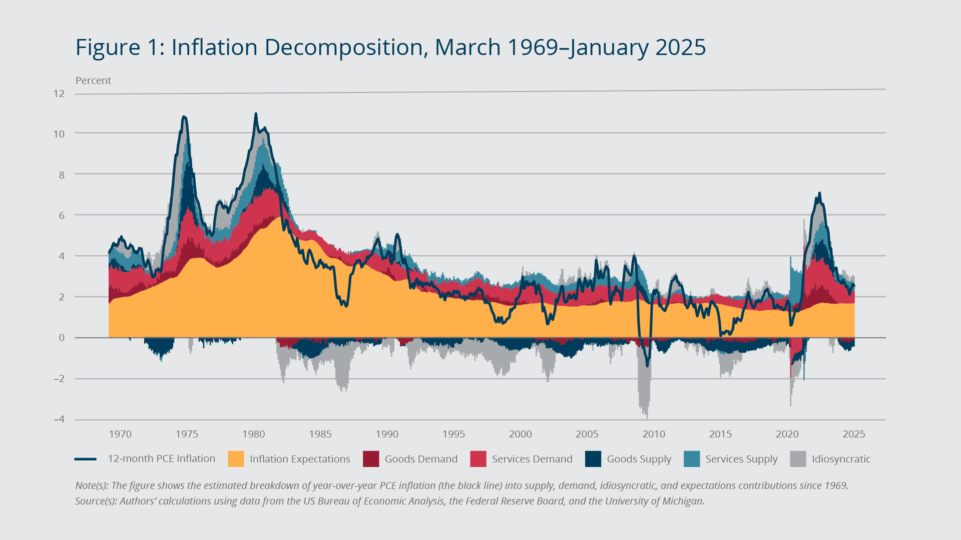
Figure 1 shows our decomposition of year-over-year PCE inflation (the black line). Note that contracting goods supply (the dark blue area) significantly contributed to the inflation surge of the 1970s and early 1980s. Starting in the mid-1980s, goods supply began expanding, applying downward pressure on prices on balance, a pattern that prevailed until the post-pandemic surge in inflation. The persistent downward price pressure from goods supply that emerged in the latter part of the 1980s is consistent with increasing globalization over the subsequent three decades, during which goods manufacturers shifted to the lowest-cost labor markets. As a result, goods supply became a sustained source of disinflationary pressures. Services demand (the light red area), by contrast, has been a consistent source of inflationary pressures since at least the early 1970s.

Note also that the inflation expectations component (the orange area) has been stable since the mid-1990s and barely budged during the recent spike in inflation. This pattern stands in sharp contrast to the one that prevailed during the Great Inflation of the 1970s and early 1980s, when inflation expectations’ contribution to upward price pressures was much more significant and persistent. The difference between the two periods reflects the Federal Reserve’s credible commitment to price stability following the so-called Volcker disinflation of the early 1980s—when an aggressive policy response broke the back of inflation—underscoring the benefits of stable long-term inflation expectations.

While these aggregate components explain much of the variation in inflation over the last five and a half decades, there is also an idiosyncratic component (the gray area in Figure 1) that significantly affects inflation dynamics. This component reflects factors specific to a particular category of goods or services and may involve sectoral demand and/or supply developments. For example, our model attributes a one-time change in energy prices that is quickly reverted and that does not spill over into other categories—a so-called relative price shock—to idiosyncratic inflation.³

Our decomposition provides novel insights into the highly unusual post-pandemic inflation episode, showing when and the extent to which it was driven by either supply or demand factors. Early in the pandemic, consumers switched en masse from spending on in-person services to goods available from online retailers. While aggregate demand remained strong, on balance, its composition changed drastically over a short period. This sudden rotation in demand was followed by severe supply-chain disruptions that were compounded by a surge in global energy prices following Russia’s invasion of Ukraine in February 2022.

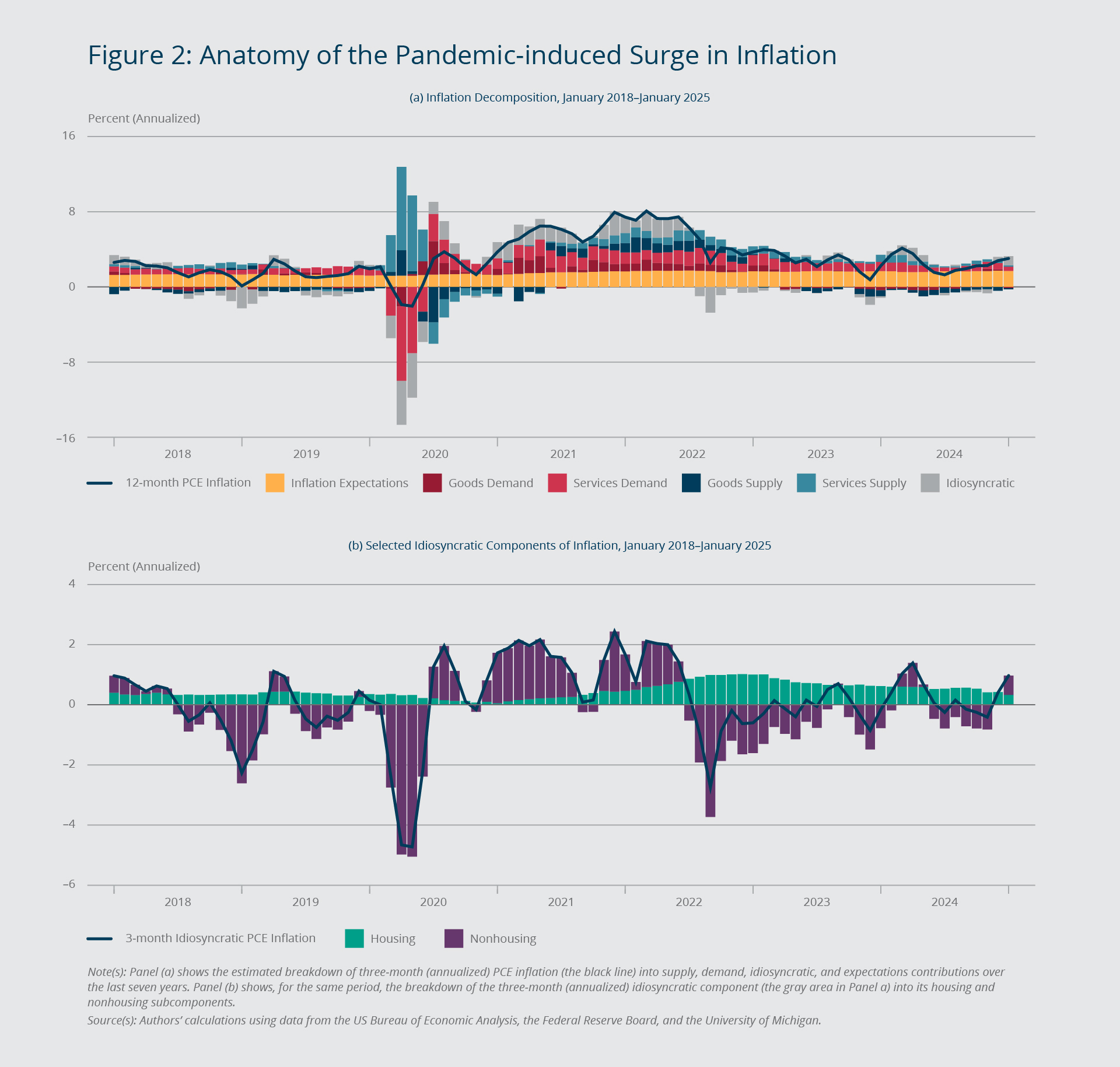
The top panel of Figure 2 zooms in on the recent period through January 2025, focusing on three-month (annualized) inflation rates to better illustrate the various phases. Over the first few months of the pandemic, as widespread business closures went into effect, aggregate demand and aggregate supply both collapsed. These two developments had opposite effects on inflation and, according to our estimates, roughly offset each other.

Supported by significant fiscal stimulus, demand-driven inflation started to surge in mid-2020 and remained elevated through 2022.⁴ Initially, the recovery of the supply side from the immediate impact of the pandemic kept total inflation at bay. However, supply conditions began to worsen in the second half of 2021 and started to boost inflation alongside the persistent and elevated demand, especially for services. Although it was declining, inflation driven by demand for services proved to be substantially more persistent than inflation related to the other aggregate components identified by our model, a result consistent with the slow resolution of labor shortages, which were especially acute in the service sector.

The bottom panel of Figure 2 focuses on idiosyncratic inflation (the gray area in the top panel) and divides this component into housing and nonhousing subcomponents. Consistent with the narrative surrounding the ongoing disinflation process, idiosyncratic housing inflation (the teal area) has been stubbornly elevated since mid-2022 and did not start to decline until the end of 2024. By contrast, idiosyncratic price developments in nonhousing consumption categories (the purple area) were putting downward pressure on prices during this period, suggesting that elevated nonhousing inflation was due primarily to aggregate supply and demand factors.

Our estimates of supply and demand inflation factors could improve the accuracy of the near-term outlook for inflation, especially at key turning points. Figure 3 shows results from a retrospective inflation forecasting exercise based on a time-series model that includes information on past inflation, labor market conditions, energy prices, and interest rates—standard predictors of inflation in forecasting models. The two forecasts shown in the left panel are based on our estimated supply and demand factors for goods and services in addition to the aforementioned standard predictors of inflation; the right panel shows two forecasts based on just the standard predictors.⁵ Each pair of forecasts includes one that uses information as of December 2020, right before inflation started to surge (red lines and red-shaded areas), and another that uses information as of March 2022, when inflation began to level off (blue lines and blue-shaded areas). The black line in each panel depicts actual year-over-year inflation.

Focusing first on the 2021 run-up in inflation (red lines), we see that incorporating the information on the demand and supply factors (left panel) captures two features of the run-up that were difficult to discern in real time. First, the forecast with the inflation factors (left panel) depicts a much more rapid surge to nearly 8 percent, resulting in a potentially long-lasting deviation from the Federal Reserve’s 2 percent target. The forecast omitting the inflation factors (right panel), by contrast, suggests a transitory spike in inflation—it is above the Fed’s target for only about six months. Second, in the forecast that incorporates our inflation factors, after the initial projected surge, the uncertainty associated with the inflation outlook (the red-shaded area) increases substantially, a potential preview of the highly unusual inflation dynamics that lay ahead. It is worth noting that the forecast’s call for a surge in inflation is driven by information on services supply; anticipation of the subsequent persistent high inflation, however, is informed by the goods supply and demand factors.⁶

Turning to the forecasts that use data up to the start of the disinflation (blue lines), we see that the forecast omitting the inflation factors (right panel) fails to anticipate the swift decline in inflation. By contrast, the projection that incorporates our inflation factors (left panel) does a remarkably good job of forecasting the ensuing disinflation. It is the goods supply factor that signals the relatively—and to many observers, surprisingly—quick decline in inflation over the subsequent 15 months.

Our framework can also provide useful insights about the ongoing disinflation process. Aggregate and disaggregated PCE inflation rates both are volatile, making it difficult to separate signal from noise, especially when considering price changes over shorter periods such as one month or three months.

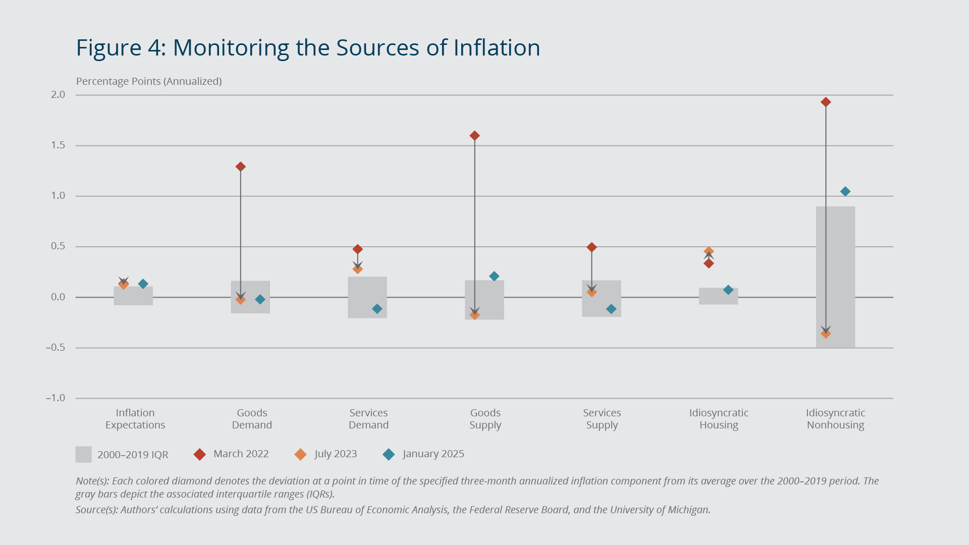
In Figure 4, the colored diamonds show deviations of the three-month (annualized) inflation components at different points of the current disinflation process from their average levels over the 2000–2019 period. The gray bars depict the typical range of deviations over this period.

In March 2022 (the red diamonds), when inflation appeared to have peaked, all supply and demand components were significantly above their typical ranges. As indicated by the black arrows, all four had moved within or close to their typical ranges by July 2023 (the orange diamonds). These aggregate sources of inflation continued to normalize over the following period and into early 2025 (the blue diamonds).

Note that idiosyncratic inflation played an important role during both the inflation surge and the subsequent disinflation. While idiosyncratic nonhousing inflation declined in line with aggregate supply and demand components from March 2022 to July 2023, idiosyncratic housing inflation continued to hover noticeably above its typical range. By January 2025, however, idiosyncratic housing inflation had returned to its typical pre-pandemic range. Idiosyncratic nonhousing inflation, on the other hand, was elevated by historical standards. All told, our decomposition suggests that as of January 2025, the remaining gap between PCE inflation and the Fed’s 2 percent target largely reflected idiosyncratic nonhousing inflation.

1. Throughout this brief, inflation refers to the growth (measured as a log difference) of the total PCE price index, which, unlike the core index, includes food and energy prices. The PCE price index is the Federal Reserve’s preferred measure of economy-wide price changes. The Federal Open Market Committee has interpreted the Fed’s price stability mandate as maintaining year-over-year PCE inflation at 2 percent. The total PCE inflation values shown in the figures are aggregated from the 51 categories of PCE used in the estimation. From the so-called Level 4 disaggregation, which includes 53 categories, we exclude the two categories with possibly negative expenditure weights: Net Expenditures Abroad by US Residents and Net Foreign Travel.
2. Formally, we use Bayesian methods to estimate a sign-restricted dynamic factor model (SiR-DFM) that allows for stochastic volatility and the presence of outliers in the idiosyncratic (that is, category-specific) inflation and consumption growth components, two prominent features of disaggregated PCE data; see Leiva-León et al. (2025) for technical details. Sign-restriction identification strategies have a long history in economics; see Fry and Pagan (2011) for a comprehensive review of the literature. Recently, Shapiro (2022, 2024) and Sheremirov (2022) apply this approach to disaggregated PCE inflation data. Our approach differs from Shapiro (2022, 2024) in three important ways. First, we separate aggregate demand and aggregate supply components from idiosyncratic demand and supply factors. Second, we separate demand- and supply-driven inflation within each consumption category in a given period, rather than classifying inflation in an entire category as purely demand or supply driven. Third, our estimation incorporates measures of inflation expectations to account for long-term trends in inflation. Specifically, we use inflation expectations from the University of Michigan’s Surveys of Consumers. This series, which measures expected inflation over the next five to 10 years, is available at a monthly frequency starting in April 1990. For the earlier period, we use long-term expected inflation from the Federal Reserve Board’s FRB/US database; see Brayton and Tinsley (1996) for details.
3. It is worth noting that from the mid-1990s to end of 2019—a period of low and stable inflation—the idiosyncratic component was an important driver of fluctuations in total inflation. During the period of high and volatile inflation in the 1970s and 1980s, by contrast, most of the volatility in total inflation was due to aggregate factors. These results are consistent with the two-regime view of inflation advanced by Borio et al. (2023).
4. The American Rescue Plan of 2021 was signed into law by President Joe Biden on March 11, 2021. Among other initiatives, this $1.9 trillion stimulus package included provisions for direct payment to households and extended unemployment benefits.
5. We start with a Bayesian vector autoregression (BVAR) forecasting model that includes PCE inflation, the unemployment rate, unit labor costs, Consumer Price Index (CPI) energy price growth, and the two-year nominal Treasury yield, which captures the stance of monetary policy. We also consider an extension of this model that includes our four estimated inflation factors (goods demand, goods supply, services demand, and services supply). At each jump-off point, the forecasts of year-over-year PCE inflation are based on the information available at the time the prediction would have been made.
6. See Leiva-León et al. (2025) for more details.

Borio, Claudio, Marco Lombardi, James Yetman, and Egon Zakrajšek. 2023. “The Two-regime View of Inflation.” Bank for International Settlements BIS Papers No. 133.

Brayton, Flint, and Peter A. Tinsley. 1996. “A Guide to FRB/US: A Macroeconomic Model of the United States.” Board of Governors of the Federal Reserve System Finance and Economics Discussion Series (FEDS) 96-42.

Federal Reserve Board. “FRB/US Data‌‌‌‌ Package.” Accessed February 13, 2025. https://www.federalreserve.gov/econres/us-models-python.htm

Fry, Renée, and Adrian Pagan. 2011. “Sign Restrictions in Structural Vector Autoregressions: A Critical Review.” Journal of Economic Literature 49(4): 938–960.

Leiva-León, Danilo, Viacheslav Sheremirov, Jenny Tang, and Egon Zakrajšek. 2025. “Inflation Factors.” Working paper.

Shapiro, Adam Hale. 2022. “How Much Do Supply and Demand Drive Inflation?” Federal Reserve Bank of San Francisco FRBSF Economic Letter 2022-15.

Shapiro, Adam Hale. 2024. “Decomposing Supply- and Demand-driven Inflation.” Journal of Money, Credit and Banking. Forthcoming.

Sheremirov, Viacheslav. 2022. “Are the Demand and Supply Channels of Inflation Persistent? Evidence from a Novel Decomposition of PCE Inflation.” Federal Reserve Bank of Boston Current Policy Perspectives. November 7